library(keras)
# classic mnist dataset
mnist <- dataset_mnist()
# training set
train_images <- mnist$train$x
train_labels <- mnist$train$y
# test set
test_images <- mnist$test$x
test_labels <- mnist$test$y
rescale so that values are in the [0, 1] interval
train_images <- array_reshape(train_images, c(60000, 28 * 28))
train_images <- train_images / 255
test_images <- array_reshape(test_images, c(10000, 28 * 28))
test_images <- test_images / 255
network architecture
network <- keras_model_sequential() %>%
    layer_dense(units = 512, activation = "relu", input_shape = c(28 * 28)) %>%
    layer_dense(units = 10, activation = "softmax")
complete our network
network %>% compile(
    # how the network update itself
    # https://keras.io/optimizers/
    optimizer = "rmsprop",
    # loss function
    # https://keras.io/losses/
    loss = "categorical_crossentropy",
    # metrics to monitor
    # https://keras.io/metrics/
    metrics = c("accuracy")
)
dummify our labels
train_labels <- to_categorical(train_labels)
test_labels <- to_categorical(test_labels)
print summary
summary(network)
## ___________________________________________________________________________
## Layer (type)                     Output Shape                  Param #
## ===========================================================================
## dense_1 (Dense)                  (None, 512)                   401920
## ___________________________________________________________________________
## dense_2 (Dense)                  (None, 10)                    5130
## ===========================================================================
## Total params: 407,050
## Trainable params: 407,050
## Non-trainable params: 0
## ___________________________________________________________________________
train the network
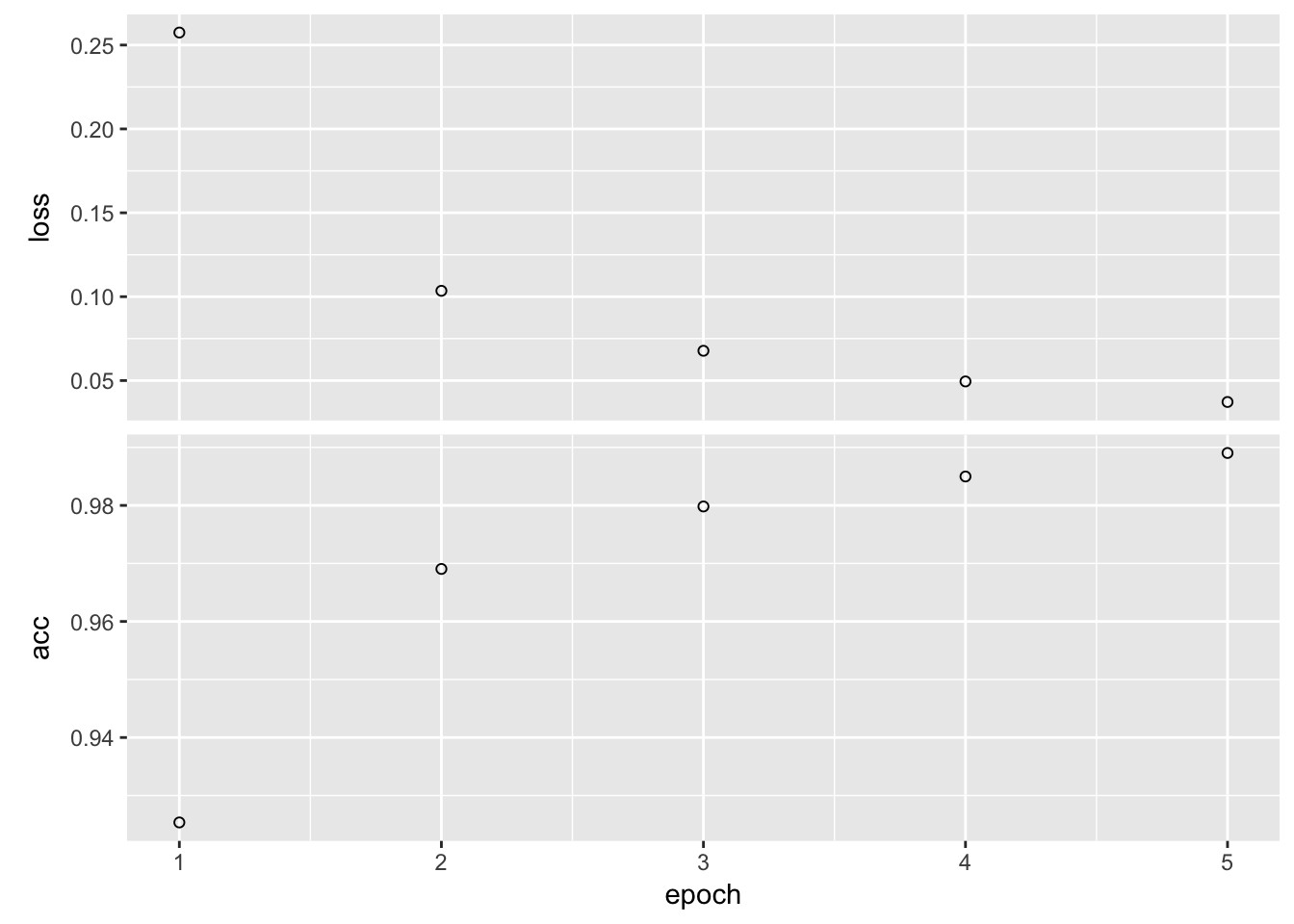
history <- network %>% fit(train_images, train_labels, epochs = 5, batch_size = 128)
plot(history)
make predictions
list(
    actual = mnist$test$y[1:10],
    preds = network %>% predict_classes(test_images[1:10, ])
)
## $actual
##  [1] 7 2 1 0 4 1 4 9 5 9
##
## $preds
##  [1] 7 2 1 0 4 1 4 9 5 9